L-flange, deterministic analysis
This tutorial performs the deterministic bolt fatigue assessment of an L-flange according to IEC 61400-6 AMD1, for a single design gap. It covers the whole chain: bolt, gap, flange segment, validity check, bolt force and moment curves, fatigue damage.
Download the full script:
lflange.py. Run it with
py lflange.py.
1. Units
PyFlange works with any consistent system of units. We use SI units and define a few factors to make the input readable:
2. Bolt, nut and bolt hole
from pyflange.bolts import StandardMetricBolt, RoundNut, standard_hole_diameter

bolt = StandardMetricBolt("M80", "10.9",
                          shank_length = 160*mm,
                          shank_diameter_ratio = "pitch",   # reduced shank
                          stud = True)
nut = RoundNut("M80")
Do = standard_hole_diameter("M80")      # 86 mm bolt hole
StandardMetricBoltcreates a bolt with ISO thread dimensions and the properties of the material grade.stud=Truemodels a stud bolt with two nuts;shank_diameter_ratio="pitch"gives a reduced shank with the diameter of the thread pitch diameter.RoundNutis a flanged round nut. UseISOHexNutfor a hexagon nut, and pass aISOFlatWasheraswasherif there is one.standard_hole_diameterreturns the standard clearance hole.
3. Design gap
The polynomial model accounts for a gap between the two flanges, caused by flatness imperfections. IEC 61400-6 AMD1 defines the design gap height as the 95% quantile of a log-normal distribution that depends on the tower diameter, the flatness tolerance and the gap length (ref. [2], 6.7.5.2):
from pyflange.stats import gap_height_distribution
from pyflange.flangesegments import Gap, shell_stiffness

D = 8000*mm                 # flange (tower) outer diameter
u_tol = 1.4*mm / 1.0        # flatness tolerance: 1.4 mm/m
gap_angle = 30*deg          # gap angle
gap_length = gap_angle * D/2

gap_dist = gap_height_distribution(D, u_tol, gap_length)
gap = Gap(height = gap_dist.ppf(0.95),   # design gap: 95% quantile
          angle = gap_angle)
For an 8 m tower with a 1.4 mm/m tolerance and a 30° gap, the design gap height is 0.89 mm. In this tutorial we check the 30° gap only. The standard requires the gap angles 30°, 60°, 90° and 120°: see Design gap angles and ED2.
4. Flange segment
The model describes one segment of the flange: the slice that contains one bolt (see Model overview and Nomenclature for the symbols).
from pyflange.flangesegments import PolynomialLFlangeSegment

n_bolts = 156               # number of bolts in the flange
R = D/2                     # shell outer radius
s = 54*mm                   # shell thickness

fseg = PolynomialLFlangeSegment(
    a = 150*mm,             # inner face of the flange to bolt axis
    b = 122*mm,             # bolt axis to shell center line
    s = s,
    t = 172*mm,             # flange thickness
    R = R,
    central_angle = 2*pi / n_bolts,

    Zg = -18044*kN / n_bolts,           # dead weight per bolt (compression)

    bolt = bolt,
    Fv = 2876*kN,                       # bolt preload before losses
    Do = Do,
    washer = None,
    nut = nut,

    gap = gap,
    tilt_angle = 0.1*deg,               # inside flange inclination

    k_shell = shell_stiffness(R, s, gap_angle),   # shell stiffness from FEA data
    PPL = 0.05,                         # 5% preload loss due to plastic strain
    DFT = 300e-6,                       # 300 um coating thickness
    settlement_factor = 0.5)            # tension tightening with re-tightening
Some parameters deserve attention:
Zgis the shell force per bolt in the unloaded state, normally the dead weight above the flange divided by the number of bolts. It is negative because it compresses the flange.Fvis the preload before losses. The losses due to settlement (DFT,settlement_factor, ref. [2], eqs. (27) and (28)) and plastic strain (PPL, ref. [2], eq. (24)) are subtracted by the model. The resulting preload is available asfseg.bolt_preload. If yourFvalready includes all losses, leavePPLandDFTat their default value of zero.k_shellis the shell stiffness. Here it is interpolated from a database of FEA results withshell_stiffness. If omitted, the simplified formula of ref. [2], eq. G.43 is used, which is conservative.tilt_angleis the inclination of the flange contact surface. A positive value (inclination towards the inside) reduces the bolt forces.E,G,s_ratio(bottom shell thickness overs) andr(fillet radius) have default values; seePolynomialLFlangeSegment.
5. Check that the model is applicable
The polynomial model of an L-flange is valid only if failure mode B (plastic hinges in the flange and in the shell) is the governing ultimate failure mode (ref. [2], eq. G.30):
mode, Zu = fseg.failure_mode(fy_sh=355*MPa, fy_fl=335*MPa)
print(f"Governing failure mode: {mode}")
print(f"Ultimate shell forces A, B, D, E [kN]: {[round(Z/kN) for Z in Zu]}")

fseg.validate(fy_sh=355*MPa, fy_fl=335*MPa)    # raises ValueError if mode B does not govern
validate() raises a ValueError if another mode governs, so a script
stops before producing results outside the validity range of the model.
6. Bolt force curve
The bolt force curve is defined by four points (ref. [2], Table G.1):
print(f"Preload after losses: {fseg.bolt_preload/kN:.0f} kN")
print(f"P1 (at rest):       Z = {fseg.shell_force_at_rest/kN:8.1f} kN   Fs = {fseg.bolt_force_at_rest/kN:7.1f} kN")
print(f"P2 (tensile ULS):   Z = {fseg.shell_force_at_tensile_ULS/kN:8.1f} kN   Fs = {fseg.bolt_force_at_tensile_ULS/kN:7.1f} kN")
print(f"P3 (small displ.):  Z = {fseg.shell_force_at_small_displacement/kN:8.1f} kN   Fs = {fseg.bolt_force_at_small_displacement/kN:7.1f} kN")
print(f"P4 (gap closed):    Z = {fseg.shell_force_at_closed_gap/kN:8.1f} kN")
Preload after losses: 2669 kN
P1 (at rest):       Z =   -115.7 kN   Fs =  2669.2 kN
P2 (tensile ULS):   Z =   1840.0 kN   Fs =  3336.6 kN
P3 (small displ.):  Z =    111.1 kN   Fs =  2677.0 kN
P4 (gap closed):    Z =   -427.5 kN
The transfer functions accept a single value or a numpy array of shell forces:
import numpy as np

Z = np.linspace(-500*kN, 1500*kN, 201)     # shell force per bolt
Fs = fseg.bolt_axial_force(Z)              # bolt axial force
Ms = fseg.bolt_bending_moment(Z)           # bolt bending moment

print(f"Fs(Z = 500 kN) = {fseg.bolt_axial_force(500*kN)/kN:.1f} kN")
print(f"Ms(Z = 500 kN) = {fseg.bolt_bending_moment(500*kN)/1000:.2f} kNm")
With matplotlib installed, the script also plots the curves:
try:
    import matplotlib.pyplot as plt
except ImportError:
    plt = None      # matplotlib is optional: py -m pip install matplotlib

if plt:
    fig, (ax1, ax2) = plt.subplots(1, 2, figsize=(10, 4))
    ax1.plot(Z/kN, Fs/kN)
    ax1.set_xlabel("Shell force Z [kN]")
    ax1.set_ylabel("Bolt axial force Fs [kN]")
    ax1.grid(True)
    ax2.plot(Z/kN, Ms/1000)
    ax2.set_xlabel("Shell force Z [kN]")
    ax2.set_ylabel("Bolt bending moment Ms [kNm]")
    ax2.grid(True)
    fig.tight_layout()
    fig.savefig("lflange-transfer-functions.png")
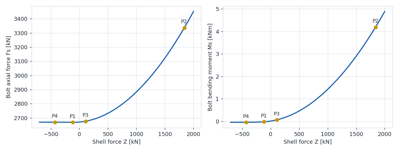
Below P1 the flange is compressed and the gap closes: at P4 it is completely closed and the bolt force stays constant. Above P1 the bolt force increases quadratically up to the ultimate state P2. P3 sets the initial slope of the curve.
7. Fatigue analysis
The fatigue loads are given as a Markov matrix of tower bending moments
at the flange. BoltFatigueAnalysis
converts them into bolt stresses through the transfer functions and computes
the damage with the IEC bolt S-N curve (detail category 50, size effect,
γM = 1.1, ref. [2], 6.7.5.4):
from pyflange.fatigue import MarkovMatrix, BoltFatigueAnalysis

# Tower bending moment Markov matrix at the flange, for 30 years
mkvm = MarkovMatrix(
    range  = np.array([ 25,  50, 100, 150, 200, 250,  300, 375, 500, 625]) * 1e6,   # N·m
    mean   = np.array([100, 100, 100, 100, 100, 100,  100, 100, 100, 100]) * 1e6,   # N·m
    cycles = np.array([3e8, 1e8, 3e7, 8e6, 2e6, 5e5, 1.5e5, 4e4, 8e3, 1e3]),
    duration = 30)                                                                 # years

fatigue = BoltFatigueAnalysis(fseg, mkvm)

print(f"S-N curve knee point: {fatigue.fatigue_curve.curves[0].DS_ref/MPa:.1f} MPa")
print(f"Damage:       {fatigue.damage:.3f}")
print(f"Fatigue life: {fatigue.fatigue_life:.1f} years")
The damage is below 1.0, so the bolts pass for the 30° gap. The bolt stress
Markov matrix is available as fatigue.bolt_mkvm, and a different S-N curve
can be passed as custom_fatigue_curve. A stress multiplication factor
(SMF) can be applied to the bolt stress ranges.
Next steps
- Check all the design gap angles: Design gap angles and ED2.
- Save this case to a JSON file and run it from the command line: Writing case files from Python.
- The meaning of each intermediate quantity: Model overview and the API reference.